Pointwise and uniform convergence in statistics and machine learning.
In this note, I want to clarify how and why the somewhat subtle distinction between pointwise and uniform convergence in probability is important for understanding the generalisation ability of a machine learning algorithm.
In this publically available lecture here [1], Larry Wasserman makes the following remark concerning pointwise and uniform convergence in probability, in context of binary classification:
“This is the subtlety that pervades everything in statistics and machine learning.”
Given that I don’t have a strong background in analysis, when I first made notes on the lecture as part of self-study in April 2020, the distinction between pointwise and uniform convergence was too nuanced for me to fully understand. Consequently I was unable to appreciate the significance of this remark.
It turns out that this distinction is highly significant for theoretical understanding of a central question in machine learning, which is:
Why does reducing training error reduce test error?
In this post, I will take the expository route of presenting an excerpt from Larry Wasserman’s lecture notes concerning the distinction between pointwise and uniform convergence, followed by brief informal arguments made in the lecture recording on why this is important in the supervised binary classification setting. I will present the queries that arose as I parsed these materials. Then I will outline empirical risk minimisation, the general framework necessary for elucidating on these queries; followed by a deeper intuitive explanation on the distinction between pointwise deviations (concentration inequalities), and uniform deviations (uniform bounds). The crux of the post will be how excess risk and generalisation error can be bounded by a uniform deviation, followed by an illustration of this principle on a finite function class. I will conclude with how this strategy relates to the subfield of empirical processes, and how it underlies more sophisticated approaches in statistical learning theory.
The illustrative context - binary classification.
The following is an excerpt from “Lecture Notes 3: Uniform Bounds” in the Carnegie Mellon university course, “36-705 Intermediate Statistics Fall 2016”. This is a compulsory course for MSc/PhD students studying machine learning. The materials were downloaded from the original course page, but as the course page has been taken down, is available at my GitHub repo [2]. I have included some comments to preserve narrative flow.
We have the following supervised learning setup for binary classification.
- We have \(N\) observed data points consisting of input-label pairs \((X_1, Y_1), ..., (X_n, Y_n)\) where \(X_i \in \mathbb{R}^d\) and \(Y_i \in \{0, 1\}\).
- Let \((X, Y)\) be a new pair, that is, we observe \(X\) and do not have \(Y\).
- We would like to predict the class label \(Y\).
- A classifier \(f\) is a function \(f: X \in \mathbb{R}^d \rightarrow Y \in \{0, 1\}\).
- When we observe \(X\) we predict \(Y\) with \(f(X)\).
The classification error, or risk, is the misclassification probability:
\[R(f) = P(Y \neq f(X))\]The training error, or empirical risk, is the fraction of errors on the observed data \((X_1, Y_1), ..., (X_n, Y_n)\):
\[\hat{R}_n(f) = \frac{1}{n} \sum^n_{i=1} \mathbb{I}(Y_i \neq f(X_i))\]Each indicator function \(\mathbb{I}(Y_i \neq f(X_i))\) can be viewed as an independent and identically distributed Bernoulli random variable \(W_i \sim \text{Bernoulli}(p)\), with mean parameter \(p\). Meaning that \(W_i\) is bounded in \([0, 1]\), and where the mean parameter \(p = \mathbb{E}[W_i]\) The consequence is that we can view the empirical risk as a sample mean \(\bar{W}_n\), and the risk as the corresponding expectation \(\mathbb{E}[W_i]\), and apply the concentration inequality of Hoeffding.
Hoeffding’s inequality, applied to the case of Bernoulli random variables \(W_i\) states that for all \(\epsilon > 0\):
\[\mathbb{P}(|\bar{W_n} - \mathbb{E}[W_i]| > \epsilon) \leq 2\exp(-2n\epsilon^2)\]Where \(\bar{W_n} = n^{-1} \sum^n_{i=1} W_i\) is the sample mean. Applying this to our specific context we have:
\[\mathbb{P}(|\hat{R}_n(f) - R(f) | > \epsilon) \leq 2\exp(-2n\epsilon^2)\]The above is a probabilistic bound on a pointwise deviation. Now this can be viewed asymptotically as a statement of pointwise convergence in probability, in the sense that:
\[\lim_{n \rightarrow \infty} P(|\hat{R}(f) - R(f) | > \epsilon) = 0\]So far so good, nothing deeply contentious so far. Here is where we start to see some more nuanced arguments:
How do we choose a classifier? In supervised learning, we start with a set of classifiers \(\mathcal{F}\). We then define \(\hat{f}\) to be a member of \(\mathcal{F}\) that minimises the training error, that is:
\[\hat{f} = \text{argmin}_{f \in \mathcal{F}} \hat{R}(f)\]For concreteness, let \(\mathcal{F}\) be the set of all linear classifiers, that is functions \(f\) taking the following form:
\[f(x) = \begin{cases} 1 \quad \text{if} \quad \theta^Tx \geq 0 \\ 0 \quad \text{if} \quad \theta^Tx < 0 \\ \end{cases}\]Where \(\theta = (\theta_1, ..., \theta_d)^T\) is a vector of parameters, that is, \(\theta \in \mathbb{R}^d\).
Although \(\hat{f}\) minimises \(\hat{R}(f)\), there is no reason to expect for it minimise \(R(f)\). Let \(f^*\) minimise the “true” error \(R(f)\). A fundamental question then is, how close is \(R( \hat{f} )\) to \(R(f^*)\)?
We will see later that \(R(\hat{f})\) is close to \(R(f^*)\) if \(\sup_{f \in \mathcal{F}} \lvert \hat{R}(f) - R(f) \rvert\) is small. So we want:
\[\mathbb{P}\left(\sup_{f \in \mathcal{F}} | \hat{R}(f) - R(f) | > \epsilon \right) \leq \text{something small}\]Which is a probabilistic bound on a uniform deviation. Asymptotically, this can be viewed as a statement concerning uniform convergence in probability. From hereon, we will use the word pointwise or uniform deviation to refer to the finite sample setting, whereas we will use pointwise or uniform convergence in probability to refer to the asymptotic setting. This is where the note excerpt ends.
Now here is a distillation of the informal argument given by Wasserman in the video lecture for why pointwise deviations/convergence in probability statements are insufficient for binary classification:
- We would like to choose a classifier \(f \in \mathcal{F}\) so as to minimise prediction error or risk \({R}(f)\).
- However, we do not know the risk \({R}(f)\), so we use an estimate of the risk, \(\hat{R}(f)\), and minimise this instead.
- The problem, however, is that we need to need to compute an estimate \(\hat{R}(f)\) of \(R(f)\) for multiple, possibly an infinite number of classifiers in \(\mathcal{F}\).
- If we do not estimate \(R(f)\) uniformly well, that is for each \(f \in \mathcal{F}\), then we cannot be sure that minimising \(\hat{R}(f)\) will result in a good classifier.
- That is, minimising \(\hat{R}(f)\) as a proxy for \(R(f)\) involves a search over the entire set of functions \(\mathcal{F}\). Whether or not this results in a good classifier in the sense of minimising risk \(R(f)\) is contingent on the proximity of our estimate \(\hat{R}(f)\) to the unknown \(R(f)\) ‘everywhere’, that is over the entire set \(\mathcal{F}.\)
Concretely, the issue is that a pointwise deviation/convergence in probability statement only allows us to bound the deviation between a single random variable \(\hat{R}(f)\) from its expectation \(R(f)\). Whereas what we really want is a uniform deviation/convergence in probability statement, that is, to bound the deviations for multiple random variables from their expectations simultaneously over an entire class of functions \(\mathcal{F}\).
There a few unresolved issues in the note excerpt which need a more thorough treatment, and these queries led me to write this post:
Do there exist other criteria for selecting \(f^*\) other than minimising training error? Is this what is done in practice?
Why is it the case that \(R(\hat{f})\) will be ‘close’ to \(R(f^*)\) given uniform convergence of \(\hat{R}(f)\) to \(R(f)\) over the entire class of functions \(\mathcal{F}\)?
Is the concentration inequality for a single classifier \(f\) applicable when applied to \(\hat{f}\), given that we estimate \(\hat{f}\) from training data?
Why are probabilistic bounds on pointwise deviations insufficient?
What is the distinction between a probabilistic bound on p+ointwise deviations and on a uniform deviation?
Empirical risk minimisation - a general framework.
It turns out that the distinction between pointwise and uniform convergence is fundamental to the workings of a procedure referred to as empirical risk minimisation (ERM), a broad framework for understanding the generalisation ability of machine learning algorithms, specifically, supervised learning problems such as regression and classification, and also unsupervised learning problems such as density estimation. Empirical risk minimisation is the framework being invoked when we select \(\hat{f}\) by minimising training error.
Many explicitly associate ERM with the well-known key papers by Vladimir Vapnik and his colleagues. In terms of where one might go about locating ERM epistemologically in the field of machine learning, a natural subfield ERM is associated with is statistical learning theory. That there is significant overlap with statistics and statistical learning theory is in the name, but also in the use of tools such as stochastic processes known as empirical processes, which I will briefly touch on towards the end of the post.
There is fairly broad consensus that the importance of uniform convergence for understanding generalisation error was highlighted by Vladimir Vapnik and Alexei Chervonenkis in the 1970s, which was later rediscovered in the 1990s. Here is an excerpt from their 1970s paper [3]:
According to the classic Bernoulli theorem, the relative frequency of an event \(A\) in a sequence of independent trials converges (in probability) to the probability of that event. In many applications, however, the need arises to judge simultaneously the probabilities of an entire class \(S\) from one and the same sample. Moreover, it is required that the relative frequency of the events converge to the probability uniformly over the entire class of events \(S\). More precisely, it is required that the maximum difference (over the class) between the relative frequency and the probability exceed a given arbitrarily small positive constant should tend to zero as the number of trials is increased indefinitely.
In order to address the queries highlighted in the previous section, it is necessary to set up the general basic framework for empirical risk minimisation. We now have the following generalisation of the note excerpt from the previous section:
- Inputs and outputs: \(X \in \mathcal{X}\), \(Y \in \mathcal{Y}\)
- Restricted class of functions: \(\mathcal{F}\)
- Loss function : \(L: (\mathcal{X} \times \mathcal{Y}) \times \mathcal{F} \rightarrow \mathbb{R}\)
- Functions/hypotheses: Each function \(f \in \mathcal{F}\) maps from \(\mathcal{X}\) to \(\mathcal{Y}\)
- True underlying data-generating joint distribution \(p^*\) over input-output space \((\mathcal{X}, \mathcal{Y})\), which is unknown.
- Training data drawn from the unknown distribution \(p^*\), that is, \((X_1, Y_1), ...., (X_n, Y_n) \sim p^*\)
The risk (also known as the expected risk, test error, generalisation error) is the loss that \(f\) incurs on a new out-of-sample test example \((X, Y)\) in expectation:
\[R(f) = \mathbb{E}_{(X, Y) \sim p^*}[L(X, Y), f)]\]The risk minimiser \(f^*\) is any function in the function class \(\mathcal{F}\) that minimises the risk:
\[f^* = \text{argmin}_{f \in \mathcal{F}} R(f)\]Evidently, the lower the expected risk, the better the generalisation ability. Is it possible to minimise the expected risk? That is, is it possible to achieve the lowest possible expected risk \(R(f^*)?\) For the most the part, this is not possible, and its role is as a theoretical benchmark.
We now define the empirical counterparts of the above. The empirical risk (also known as training error) of a function \(f \in \mathcal{F}\) is the average in-sample loss over the training data:
\[\hat{R}_n(f) = \frac{1}{n} \sum^n_{i=1} L((X_i, Y_i), f)\]The empirical risk minimiser is any function \(\hat{f}\) that minimises the empirical risk:
\[\hat{f} = \text{argmin}_{f \in \mathcal{F}} \space \hat{R}_n(f)\]Some clarity is warranted concerning each of the entities we have defined:
- For a fixed, arbitrary function \(f \in \mathcal{F}\), \(\hat{R}_n(f)\) is a sample average with mean \(R(f)\).
- The empirical risk minimiser \(\hat{f}\) is a random variable, as it depends on the training examples, albeit in a somewhat non-trivial way which will later be qualified.
- The expected risk minimiser \(f^*\) is treated in a frequentist sense - it is a fixed unknown quantity.
- Hence the empirical risk \(\hat{R}(f)\) is a random variable for each \(f \in \mathcal{F}\), but the expected risk \(R(f)\) is not a random variable, but a fixed constant, albeit unknown.
- Both the empirical risk and risk can be viewed as functionals.
Furthermore, the function class \(\mathcal{F}\) is restricted because if we were to allow \(\mathcal{F}\) to be all possible functions, then the “empirical risk minimiser” would be trivially attained by selecting \(\hat{f}\) to be a function that is zero everywhere, except at \(X_i\), where it takes the value \(Y_i\). This would amount to pure interpolation of the training data, without regard for generalisation, and hence is not suited to our purposes. In practice, the function class \(\mathcal{F}\) is restricted in advance to be say a parametric statistical model, decision trees, linear functions, polynomial functions etc.
We can now frame our theoretical queries in terms of differences involving the above quantities.
How do expected and empirical risk compare for the empirical risk minimiser \(\hat{f}\)? The difference in the expected risk and empirical risk evaluated at the empirical risk minimiser we will refer to the as the generalisation error (also generalisation gap, error bound):
\[R(\hat{f}) - \hat{R}_n(\hat{f})\]How well is the empirical risk minimiser \(\hat{f}\) doing with respect to the best in the function class \(f^*\)? The difference between the expected risk of the empirical risk minimiser and the lowest expected risk, that is, error bound relative to the best in the class, is the excess risk:
\[R(\hat{f}) - R(f^*)\]For this post, but also more broadly in statistical learning theory, the excess risk is the primary quantity of interest.
Bounding excess risk with concentration inequalities - the issue.
We are now interested in specifying a probabilistic bound on the excess risk. The excess risk is a random quantity, due to a dependence of \(R(\hat{f})\) on the training examples through \(\hat{f}\), whilst \(f^*\) is unknown but fixed. To that end, we require bounds of the following form:
\[\mathbb{P}(\lvert R(\hat{f}) - R(f^*) \rvert > \epsilon) \leq \delta\]We can decompose the excess risk in terms of that which we can observe, that is, the empirical risk:
\[R(\hat{f}) - R(f^*) = \underbrace{[R(\hat{f}) - \hat{R}_n(\hat{f})]}_{(i)} + \underbrace{[\hat{R}_n(\hat{f}) - \hat{R}_n(f^*)]}_{(ii) \space \leq \space 0} + \underbrace{[\hat{R}_n(f^*) - R(f^*)]}_{(iii)}\]Before scrutinising each term, note that is one possible decomposition of the excess risk, and that other versions exist depending on our theoeritcal motivations. Now term \((ii)\) is will be non-positive, by definition of the empirical risk minimiser \(f^*\) as that which minimises empirical risk. Term \((iii)\), which is an error bound, and because \(f^*\) is a fixed function in \(\mathcal{F}\), we can bound it using a concentration inequality e.g. Hoeffding:
\[P(\lvert \hat{R}_n(f^*) - R(f^*) \rvert \geq \epsilon) \leq 2\exp(-2n\epsilon^2)\]We might be tempted to use similarly use a concentration inequality to bound term \((i)\) in the same way we have done above, however, that is not possible, and the reason why relates to the following previously posed question:
Is the concentration inequality for a single classifier \(f\) applicable when applied to \(\hat{f}\), given that we estimate \(\hat{f}\) from training data?
The issue here is that \(\hat{f}\), which is the empirical risk minimiser, depends on the training data, and so the empirical risk evaluated at \(\hat{f}\), which is
\[\hat{R}_n(\hat{f}) = \frac{1}{n} \sum^n_{i=1} \mathbb{I}(Y_i \neq \hat{f}(X_i))\]is no longer a sum of I.I.D. random variables. Hence we cannot invoke a concentration inequality, and the primary reason for this is dependence of \(\hat{f}\) on the training data.
Empirical risk minimisation - why concentration inequalities are insufficient.
Why are probabilistic pointwise deviations insufficient?
Let’s temporarily set aside the issue of bounding excess risk, and dig more deeply into why a concentration inequality on a single fixed function \(f \in \mathcal{F}\) is by itself, insufficient for the purposes of empirical risk minimisation. This extends to why even applying a concentration inequality to every function \(f \in \mathcal{F}\) is also insufficient. In short, the answer is because concentration inequalities are probabilistic bounds on pointwise deviations, whereas what is required for empirical risk minimisation is a probabilistic bound on a uniform deviation. The followin section adapts and supplements a tutorial on statistical learning theory by Olivier Bousquet et al. (2004) [4] to develop intuition on why this is the case.
We will first need to rewrite our concentration inequality, so starting with
\[P(\lvert \hat{R}_n(f) - R(f) \rvert \geq \epsilon) \leq 2\exp(-2n\epsilon^2)\]we set the R.H.S. equal to some \(\delta > 0\) and request the value of \(\epsilon(\delta)\) that will make the inequality true. We find that the inequality will hold true when
\[\epsilon = \sqrt{\frac{\ln(2 / \delta)}{2n}}\]Now rewriting in terms of the complementary event \(E'_f = \{ \lvert \hat{R}_n(f) - R(f) \rvert \leq \epsilon \}\), our concentration inequality can be restated as the following:
\[P \left(\lvert \hat{R}_n(f) - R(f) \rvert \leq \sqrt{\frac{\ln(2 / \delta)}{2n}} \right) \geq 1 - \delta\]Where \(\epsilon\) is often referred to as accuracy, and \(1 - \delta\) is referred to as confidence. The limitations of the above statement can be seen through an appropriate interpretation. The above states that to each fixed function \(f \in \mathcal{F}\), there will be an associated set \(S_f =\{\mathcal{D}^{(1)}, ..., \mathcal{D}^{(s)} \}\) consisting of \(s\) size \(n\) training datasets \(\mathcal{D}^{(s)}\) which satisfy the inequality \(\hat{R}_n(f) - R(f) \leq \sqrt{\ln(2 / \delta)/2n}\). And this set \(S_f\) of training samples has measure \(\mathbb{P}(S_f) \geq 1 -\delta\).
The crucial limitation here is that each of these sets \(S_f\) will in general be different, for different functions in the function class \(\mathcal{F}\).
To accompany the visualisations below, this same point can be framed in a slightly different way. For a particular training data set \(\mathcal{D} = (x_1, y_1), ..., (x_n, y_n)\) that has been observed, only for some of the functions in \(\mathcal{F}\) will it be the case that the deviation between the empirical risk and risk will lie in the interval \(\left[ - \sqrt{\ln(2 / \delta)/2n}, \sqrt{\ln(2 / \delta) /2n} \right]\). Where we have used the notational distinction between a random variable \(X_i\) and its realisation \(x_i\) to emphasise that we are dealing with a particular training data set.
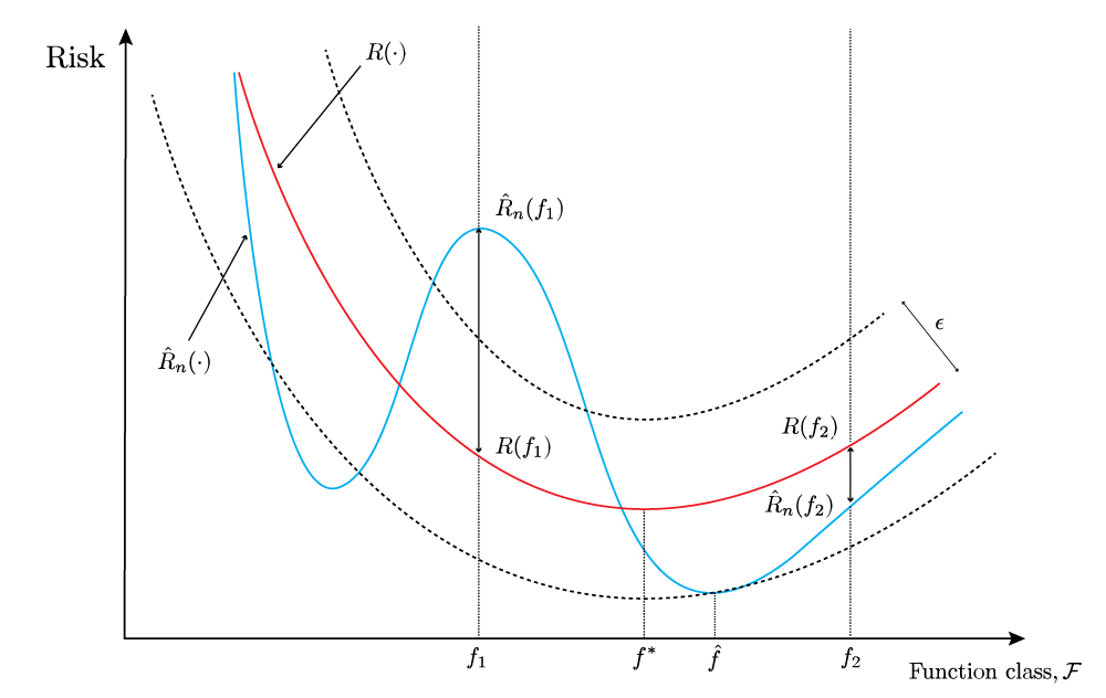
This first point can be seen in figure 1 above. The vertical slice of the plot at an arbitrary function \(f_1\) shows that for this particular training data set, the absolute deviation between the empirical risk \(\hat{R}_n(f_1)\) and risk \(R(f_1)\) exceeds \(\epsilon\). However, for the same data set, but evaluated at a different function \(f_2\), the absolute deviation does not exceed \(\epsilon\).
The second point to observe is that the probability bound supplied by a concentration inequality for a fixed function \(f\) is only applicable to an individual vertical slice of the plot. In the sense that it is a probabilistic description of the vertical distance between two points on the blue and red curves - hence a pointwise deviation. Where a point on the blue curve represents the realisation of the random variable \(\hat{R}_n(f)\) at \(f\), and where a point on the red curve is the risk \(R(f)\) at \(f\), a fixed constant.
Furthemore, the stochasticity in this plot arises from the training data \(\mathcal{D}\), on which only the observed empirical risk \(\hat{R}_n(\cdot)\) is dependent; the unobserved risk \(R(\cdot)\) on the other hand is not, and will be fixed across different training data sets.
In terms of the figure, a consequence is that for each different training data set \(\mathcal{D}\), the empirical risk \(\hat{R}_n(\cdot)\), the blue line, will have a correspondingly different shape, whilst the risk \(R(\cdot)\), the red line, will be the same. Now consider another situation that might be observed when a new training data set is drawn:
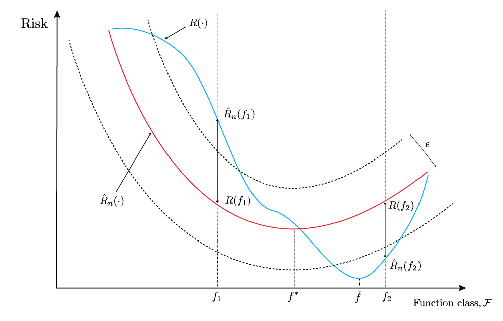
Notice that in figure 2 above, for this new training data set, the absolute deviation for the same two arbitrary functions \(f_1\) and \(f_2\) exceeds \(\epsilon\). Equally, if we were to draw another training data set, yielding a different blue curve \(\hat{R}_n(\cdot)\), we might observe that absolute deviations at these same two arbitrary functions \(f_1\) and \(f_2\) might both not exceed \(\epsilon\).
Why is this insufficient for empirical risk minimisation? As a first pass, one way of illustrating this is by going back to the fact that empirical risk minimisation is a procedure that selects a suitable function \(f\) from the entire function class \(\mathcal{F}\), resulting in the empirical risk minimiser \(\hat{f}\). This is shown as the minimum point of the blue curves in the figures. For a particular training data set \(\mathcal{D}\), we do not know what function \(f\) will be selected by ERM to be \(\hat{f}\) in advance. With only a probabilistic guarantee on the behaviour of a pointwise deviation at a fixed \(f \in \mathcal{F}\), there is no guarantee that the ERM procedure will select a function \(\hat{f}\) for which the empirical risk \(\hat{R}_n(f)\) is within an additive error bound \(\pm \epsilon\) of the risk \(R(f)\). Let’s now take this further.
Would applying a concentration inequality to every function \(f \in \mathcal{F}\), thereby bounding every individual absolute distance, \(\lvert \hat{R}_n(f) - R(f) \rvert\) alleviate the insufficiency?
Temporarily setting aside broader issues of whether the function class \(\mathcal{F}\) is countable, that is, assuming that it is indeed countable, this would be an improvement, but by itself would still be insufficient. Even though we would now have probabilistic bounds on pointwise deviations on every \(f \in \mathcal{F}\), we would still be in the realm of pointwise deviations, though applied to every function in the entire function class \(\mathcal{F}\)
To make this more precise, this amounts to asking whether the following would be sufficient for our purposes:
\[P \left(\lvert \hat{R}_n(f) - R(f) \rvert \leq \sqrt{\frac{\ln(2 / \delta)}{2n}} \right) \geq 1 - \delta \quad ,\forall \space f \in \mathcal{F}\]The answer is that in the limited case of finite function classes, this is a necessary step, but it is not sufficient. That is because we still not have gotten around the issue that we identified earlier, which is that for every function \(f \in \mathcal{F}\), the set of training data sets \(S_f\) for which the above concentration inequality holds, will differ for different functions \(f \in \mathcal{F}\). This will be addressed in more detail, and more appropriately in the next section.
Lastly, everything that has been stated so concerning the insufficiency of pointwise deviation statements also holds in the asymptotic case. In this case, finite-sample concentration inequalities can be converted from probabilistic bounds on pointwise deviations, into statements about pointwise convergence in proabibility. Visually, we can envisage that as we draw more and more training data observations, \(n \rightarrow \infty\), and the probability density function of the pointwise absolute deviation \(\lvert \hat{R}_n(f) - R(f) \rvert\) for a specific function \(f \in \mathcal{F}\), that is a vertical slice of the figure, becomes increasingly concentrated around 0.
To summarise this section, the key take aways from the figures and discussion are that:
- A single concentration inequality is a statement concerning a pointwise deviation, that is, a vertical distance on the plots above.
- Setting aside whether \(\mathcal{F}\) is countable, invoking concentration inequalities for every \(f \in \mathcal{F}\) would still qualtitatively constitute statements about pointwise deviations, albeit many pointwise deviation statements.
- Understanding empirical risk minimisation and generalisation error; and bounding excess risk requires a qualitatively stronger statement, that is, a bound on a uniform deviation.
- The concerns highlighted carry over to the asymptotic case, where concentration inequalities are pointwise convergence probability in statements, whereas uniform convergence in probability statements are required.
Empirical risk minimisation - the need for uniform deviations.
What is the distinction between a probabilistic bound on pointwise deviations and on a uniform deviation?
Continuing from before, we might now ask, in what sense is a probabilistic statement about a uniform deviation qualitatively stronger than multiple probabilistic statements about pointwise deviations?
To illustrate this, we will rely on an informal visual presentation and some hand-waving to tease out the similarities and differences, before getting to a more formal description. Here is a figure to illustrate the uniform deviation regime:
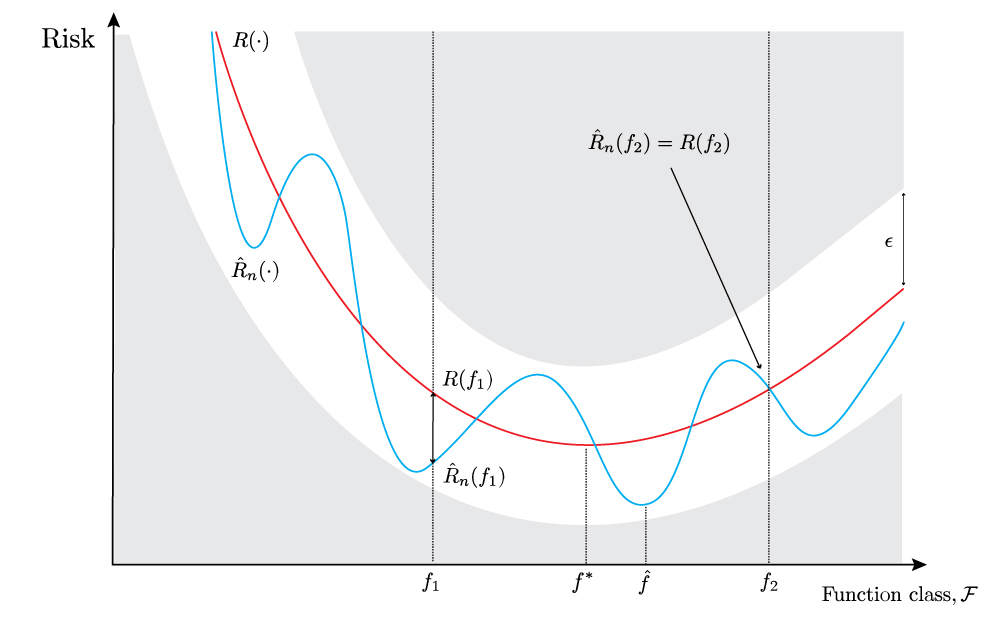
The above figure is similar to the previous two figures in the following respect - we can see that the pointwise absolute deviations are still marked for the same arbitrary functions \(f_1\) and \(f_2\). In both cases, the absolute deviations are within the white additive error band, and further, in the case of \(f_2\), the empirical risk and risk are exactly equal. This is not a feature of the uniform convergence regime per se, rather, is just an artefact of the particular training data set we have drawn, and could plausibly have occurred in the previous two figures also.
However, the key difference is that the entire area outside the white additive error band is now shaded grey. This visual difference is not to suggest anything signficant has changed, rather, to invite one to pose a different question, and thereby look at the problem in a different way. Imagine that we now ask a different question.
What is the probability that the entire blue curve, the empirical risk \(\hat{R}_n(\cdot)\), lies within the white additive error band of width \(2 \epsilon\), that is, in the interval \([R(\cdot) -\epsilon, R(\cdot) + \epsilon]\)?
This is clearly different from the previous two figures in that we are now not enquiring about a pointwise absolute deviation, that is, a vertical distance between a pair of points on the blue curve and red curve at a particular function \(f\). Rather, the enquiry about whether the blue curve lies within the white additive error band is implicitly an enquiry about the proximity of the entire blue curve to the red curve, that is, a uniform deviation over the entire function class \(\mathcal{F}\).
However, there is a somewhat more slippery distinction to make that may not be satisfactorily settled just by looking at figure 3. And that is the distinction, in terms of the figures, between bounding the individual vertical distances between every pair of points on the red and blue curve, and bounding the proximity of the entire blue curve from the red curve. Within the confines of what the figures visually articulate, this might seem like a distinction without a difference.
With the reservation that we may now be pushing the representational capacity of the figures to their limits, perhaps we could tentatively say that we need to find a way to ‘glue together’ a series of individual bounds on pointwise deviations, represented as unrelated vertical slices, into one coherent bound on a uniform deviation, represented as continuous band of white space in figure 3. However, this is tenuous, so let’s aim at a more formal description.
Formally, the distinction between bounding pointwise deviations for every function \(f \in \mathcal{F}\), and bounding a uniform deviation over the entire function class \(\mathcal{F}\) is best addressed from a probabilistic perspective. Fundamentally, the distinction is to do with the nature of the stochastic event(s) that a concentration inequality, as a pointwise deviation statement, can describe.
Resuming the argument from where we left off in the previous section, recall that for every function \(f\), the associated concentration inequality allows us to bound the probability of drawing a set \(S_f\) of training samples for which it is the case that \(\lvert \hat{R}_n(f) - R(f) \lvert\leq \sqrt{\ln(2 / \delta) / 2n}\), and that these sets \(S_f\) will in general be different for different functions \(f \in \mathcal{F}\). Even with a probabilistic bound on the pointwise deviation for every \(f \in \mathcal{F}\), these remain a series of individual bounds on individual random variables from their respective means.
In enquiring whether we can bound the probability that the entire blue curve, the empirical risk functional \(\hat{R}_n(\cdot)\), lies within a common additive error band \([R(\cdot) -\epsilon, R(\cdot) + \epsilon]\), the nature of our sample space and the stochastic event we are considering has changed. In this case, the sample space \(\Omega\) of possible outcomes is now the entire space of possible blue empirical risk functional curves \(\hat{R}_n(\cdot)\) for a given function class \(\mathcal{F}\). The stochastic event of interest \(S\) whose probability we wish to bound is now all the blue empirical risk functional curves which lie in the common white additive error band \([R(\cdot) -\epsilon, R(\cdot) + \epsilon]\).
Equivalently, this amounts to bounding the probability \(\mathbb{P}(S)\) of drawing a set \(S\) of training samples, where this set \(S\) is no longer indexed to an individual function \(f\), but satisfies the condition that for every function \(f \in \mathcal{F}\), the absolute deviation \(\lvert \hat{R}_n(f) - R(f) \rvert\) lies in the common white additive error band \([-\epsilon, \epsilon]\).
The key here is that the empirical risk functional \(\hat{R}_n(\cdot)\) for a function class \(\mathcal{F}\) now consists of a collection of random variables, where each random variable \(\hat{R}_n(f)\) is now indexed by a function \(f\). To illustrate this concretely, we index a total of \(\lvert \mathcal{F} \rvert\) random variables, and so our collection \(\hat{R}_n(\cdot)\) of random variables is now:
\[\hat{R}_n(f_1), \hat{R}_n(f_2), ... , \hat{R}_n(f_{\lvert \mathcal{F} \rvert})\]We now wish to simultaneously bound the probability of the compound event that every one of these random variables is within \(\pm \epsilon\) of a corresponding collection \(R(\cdot)\) of fixed constants, that is the theoretical means
\[R(f_1), R(f_2), ...., R(f_{\lvert \mathcal{F} \rvert})\]That we are now dealing with a probabilistic bound of at least \(1 - \delta\) on one compound event with a common additive error band \([-\epsilon, \epsilon]\), is why this is a uniform bound.
Hence the crux of what is required in a uniform deviation regime is a simultaneous probabilistic bound on the deviations of a (possibly infinite) collection of random variables \(\hat{R}_n(\cdot)\) from their means \(R(\cdot)\) over the entire function class \(\mathcal{F}\). More precisely, the uniform deviation regime is concerned with finding a probabilistic bound of the form
\[\mathbb{P}\left( \forall f \in \mathcal{F}, \space \lvert \hat{R}_n(f) - R(f) \rvert \leq \epsilon \right) \geq 1 - \delta\]Notice that the subtle distinction is in the position of the qualifier \(\forall f \in \mathcal{F}\), which now resides within the probability statement. Furthermore, noting that the compound event of the absolute deviation not exceeding \(\epsilon\) for every function \(f \in \mathcal{F}\) is the same as the compound event that the maximum absolute deviation over the entire function class \(\mathcal{F}\) does not exceed \(\epsilon\), the above is equivalent to
\[\mathbb{P} \left( \sup_{f \in \mathcal{F}} \lvert \hat{R}_n(f) - R(f) \rvert \leq \epsilon \right) \geq 1 - \delta\]For expository reasons, we have chosen to speak of the difference between pointwise and uniform deviations in terms of ‘success events’. In the next sections, we will work with bounds on ‘failure events’, that is, the complementary event that the maximum absolute deviation over \(\mathcal{F}\) exceeds \(\epsilon\), which is
\[\mathbb{P} \left( \sup_{f \in \mathcal{F}} \lvert \hat{R}_n(f) - R(f) \rvert \geq \epsilon \right) \leq \delta\]In this case, care needs to be taken with how this should be interpreted, and because I spent around half a week confused by this point, I will include its interpretation here. To express this compound event in terms of a series of pointwise deviation failure events, notice that if the maximum absolute deviation is greater than \(\epsilon\), then we can conclude that there exists at least one function \(f \in \mathcal{F}\) whose absolute deviation exceeds \(\epsilon\), and so the above is equivalent to
\[\mathbb{P} \left( \exists f \in \mathcal{F} : \lvert \hat{R}_n(f) - R(f) \rvert \geq \epsilon \right) \leq \delta\]For pointwise and uniform deviation failure events, we do not speak of ‘trapping probability in some interval \([-\epsilon, \epsilon]\) with high confidence’, i.e. at least \(1 - \delta\). Rather, we correspondingly speak of ‘bounding the tail probability’ outside the interval \([-\epsilon, \epsilon]\) such that is small i.e. less than \(\delta\).
Bounding the excess risk through a uniform deviation.
Having done a fair amount of visual hand-waving, let’s see more formally how to bound the excess risk with a uniform deviation. Returning to our original decomposition of the excess risk:
\[\begin{aligned} R(\hat{f}) - R(f^*) &= [R(\hat{f}) - \hat{R}_n(\hat{f})] + [\hat{R}_n(\hat{f}) - \hat{R}_n(f^*)] + [\hat{R}_n(f^*) - R(f^*)] \\ & \leq \lvert R(\hat{f}) - \hat{R}_n(\hat{f}) \rvert + 0 + \lvert \hat{R}_n(f^*) - R(f^*) \rvert \\ & \leq \sup_{f \in \mathcal{F}} \lvert R(f) - \hat{R}_n(f) \rvert + \sup_{f \in \mathcal{F}} \lvert \hat{R}_n(f) - R(f) \rvert \\ & \leq 2 \cdot \sup_{f \in \mathcal{F}} \lvert \hat{R}_n(f) - R(f) \rvert \\ \end{aligned}\]Where in the 2nd line we have used the fact that \(x \leq \lvert x \rvert\) for \(x \in \mathbb{R}\), and in the 3rd line, we have used the definition of the supremum. Now if we can control the term on the RHS, through a bound, then we can control the excess risk. Intuitively, we will have bounded the risk of the empirical risk minimiser \(\hat{f}\) by the “worst-case” function possible from the function class \(\mathcal{F}\).
Now due to the inequality, the occurrence of the event \(A = \{ R(\hat{f}) - R(f^*) \geq \epsilon \}\) means that the event \(B = \{\sup_{f \in \mathcal{F}} \lvert \hat{R}_n(f) - R(f) \rvert \geq \epsilon / 2\}\) simultaneously occurs, yielding the following:
\[\mathbb{P}(R(\hat{f}) - R(f^*) \geq \epsilon) \leq \mathbb{P} \left(\sup_{f \in \mathcal{F}} \lvert \hat{R}_n(f) - R(f) \rvert \geq \frac{\epsilon}{2}\right)\]This is an important statement. Explicitly, it states that the tail probability of the excess risk \(\hat{R}(f) - R(f^*)\) is bounded by the tail probability of the uniform deviation \(\sup_{f \in \mathcal{F}} \lvert \hat{R}_n(f) - R(f) \rvert\).
This suggests that if we can further bound the tail probability of the uniform deviation over the entire function class \(\mathcal{F}\), then we can also bound the tail probability of the excess risk. That is we want to find bounds of the following form:
\[\mathbb{P} \left( \sup_{f \in \mathcal{F}} \lvert \hat{R}_n(f) - R(f) \rvert \geq \frac{\epsilon}{2}\right) \leq \delta\]Previously, we examined how a bound on the excess risk could not be dealt with due to the dependence of the empirical risk minimiser \(\hat{f}\) on the training data, which meant that we could not apply a concentration inequality to bound the pointwise absolute deviation evaluated at \(\hat{f}\). The above suggests that we can circumvent this issue of dependence if we can probabilistically bound a qualitatively stronger event, that is, a uniform deviation over the entire function class \(\mathcal{F}\). Furthermore, in terms of empirical risk minimisation, if we can bound the uniform deviation over the entire function class \(\mathcal{F}\), then no matter what \(\hat{f}\) that is selected by ERM, we know by the arguments in the excess risk decomposition that the pointwise deviation of the problematic \(\lvert R(\hat{f}) - \hat{R}_n(\hat{f}) \rvert\) will also automatically be bounded.
As so far our discussion has been somewhat abstract, the points we have made can best be illustrated through a proof example.
Bounding the excess risk for a finite function class.
Let’s see how to bound the excess risk for the simple case of binary linear classification where the function class \(\mathcal{F}\) is finite. This is already covered excellently in 36-705. But I have included the proof here because I wish to explicitly show how bounding a uniform deviation is central to the proof strategy, and how this strategy is the bedrock of understanding more complex examples in statistical learning theory.
First however, some clarity on what this finite function class restriction entails is warranted. In the standard setting of binary linear classification, such as the note excerpt in the beginning of the post, we assume that the function class \(\mathcal{F}\) consists of all possible linear classifier functions \(f(x) = \mathbb{I}(\theta^Tx \geq 0)\), parametrised by \(\theta \in \Theta\), where the parameter space \(\Theta\) is taken to be \(\mathbb{R}^d\). Indexing each function \(f \in \mathcal{F}\) by a value of the parameter \(\theta \in \Theta\), the class of all linear classifiers \(\mathcal{F}\) will be uncountable, because \(\Theta = \mathbb{R}^d\) is uncountable.
Consequently, the condition that the set of linear classifiers \(\mathcal{F}\) is finite, that is, \(\lvert \mathcal{F} \rvert < \infty\), can be viewed parametrically as restricting the parameter space \(\Theta\) such that \(\theta\) can only take finitely many values. In the binary classication case, we use zero-one loss \(L((X, Y), f) = \mathbb{I}(Y \neq f(X))\), and the theorem we would like to prove is the following:
Theorem: For a finite function class \(\mathcal{F}\), where \(\lvert \mathcal{F} \rvert < \infty\), and binary zero-one loss, with probability at least \(1 - \delta\),
\[R(\hat{f}) - R(f^*) \leq \sqrt{\frac{2(\log \lvert \mathcal{F} \rvert + \log (2 / \delta))}{n}}\]
The proof proceeds in 3 steps.
Step 1. Concentration of measure for a fixed function \(f\).
For a fixed, non-random \(f \in \mathcal{F}\), that is, excluding the empirical risk minimiser \(\hat{f}\), Hoeffding’s inequality states that
\[\mathbb{P} \left( \lvert \hat{R}_n(f) - R(f) \rvert \geq \frac{\epsilon}{2} \right) \leq 2 \exp \left(-\frac{n \epsilon^2}{2} \right)\]Step 2. Bound the uniform deviation using the union bound.
Given that \(\mathcal{F}\) is a finite function class, defining the event \(E_f = \{ \lvert \hat{R}_n(f) - R(f) \rvert \geq \epsilon / 2 \}\), we can apply the union bound. This states that for a finite or countable set of events, \(E_1, ..., E_{\lvert \mathcal{F} \rvert}\), we have \(\mathbb{P}\left( \bigcup_{f \in \mathcal{F}} E_f \right) \leq \sum_{f \in \mathcal{F}} \mathbb{P}(E_f)\).
\[\begin{aligned} \mathbb{P}\left( \sup_{f \in \mathcal{F}} \lvert \hat{R}_n(f) - R(f) \rvert \geq \frac{\epsilon}{2}\right) &= \mathbb{P} \left( \exists {f \in \mathcal{F}} : \lvert \hat{R}_n(f) - R(f) \rvert \geq \epsilon / 2 \right) \\ &= \mathbb{P} \left( \bigcup_{f \in \mathcal{F}} \left \{ \lvert \hat{R}_n(f) - R(f) \rvert \geq \epsilon / 2 \right\} \right) \\ & \leq \sum_{f \in \mathcal{F}} \mathbb{P} \left( \lvert \hat{R}_n(f) - R(f) \rvert \geq \epsilon / 2\right) \\ & \leq 2 \lvert \mathcal{F} \rvert \exp \left( \frac{-n\epsilon^2}{2}\right) \\ \end{aligned}\]Invoking the union bound has allowed us to bound the tail probability of the uniform deviation over the entire function class \(\mathcal{F}\), and this is done by using the above concentration inequality to bound the tail probability of absolute deviations of the empirical risk from the risk for every function \(f \in \mathcal{F}\). In the informal terms used when describing the figures, the union bound acts like ‘glue’ - it relates individual concentration inequalities about pointwise deviations for every \(f \in \mathcal{F}\) to a uniform deviation over the entire function class \(\mathcal{F}\). This only works for the limited setting of finite function classes, otherwise we would have to evaluate an infinite sum in getting to the final inequality.
Step 3. Bound the one-sided tail probability on the excess risk.
We now use the key result established in the previous section to bound the one-sided tail probability on the excess risk using the bound on the uniform deviation.
\[\begin{aligned} \mathbb{P}(R(\hat{f}) - R(f^*) \geq \epsilon) &\leq \mathbb{P}\left( \sup_{f \in \mathcal{F}} \lvert \hat{R}_n(f) - R(f) \rvert \geq \frac{\epsilon}{2}\right) \\ & \leq 2 \lvert \mathcal{F} \rvert \exp \left( \frac{-n\epsilon^2}{2}\right) \\ \end{aligned}\]By setting \(\delta = 2 \lvert \mathcal{F} \rvert \exp (-n\epsilon^2 / 2)\), and rearranging for \(\epsilon(\delta)\), we have that
\[\epsilon = \sqrt{\frac{2 (\log \lvert \mathcal{F} \rvert + \log(2 / \delta) )}{n}}\]Rewriting in terms of complementary events, we have that:
\[\mathbb{P} \left( R(\hat{f}) - R(f^*) \leq \sqrt{\frac{2 (\log \lvert \mathcal{F} \rvert + \log(2 / \delta) )}{n}} \right) \geq 1 - \delta\]Which concludes the proof.
Some closing remarks concerning the proof are in order, which assumes familiarity with stochastic order notation. Notice that by itself, the concentration of measure inequality of Hoeffding in step 1 tells us that for a fixed \(f \in \mathcal{F}\):
\[\hat{R}_n(f) - R(f) = o_P(1) = O_P \left(\frac{1}{\sqrt{n}} \right)\]Where we have omitted constant factors and also \(\ln(2 / \delta)\), which is in general small, to get \(O_P(1 / \sqrt{n})\).
Furthermore, a consequence of step 2 is that over the entire function class \(\mathcal{F}\):
\[\sup_{f \in \mathcal{F}} \lvert \hat{R}_n(f) - R(f) \rvert = O_P \left(\sqrt{\frac{\ln \lvert \mathcal{F} \rvert}{n}} \right)\]The key interpretation is that the extra \(\sqrt{\ln \lvert \mathcal{F} \rvert}\) term represents the ‘price incurred’ in going from a pointwise deviation to a stronger uniform deviation. This extra term is dependent on the cardinality of the function class \(\lvert \mathcal{F} \rvert\), and can be viewed as a measure of the ‘complexity’ of the function class, although this latter point is difficult to appreciate without further results (see below on VC theory). Furthermore, if the function class \(\mathcal{F}\) is not too large, relative to the number of samples \(n\), then the uniform deviation is also \(o_P(1)\).
Lastly, similar arguments can be made about the excess risk \(R(\hat{f}) - R(f^*)\) being \(o_P(1)\) and \(O_P(\sqrt{\ln \lvert \mathcal{F} \rvert / n})\).
Hopefully this now concretely clarifies how one way of studying the behaviour of excess risk is by considering uniform deviations of the empirical risk and risk over an entire function class \(\mathcal{F}\).
Relationship to empirical processes.
It turns out that the study of uniform deviations and uniform convergence is one of the central preoccupations of a subfield of statistics and probability known as empirical process theory. To motivate further reading in this area, I’ve outlined an excerpt from Bodhissatva Sen’s following notes here.
For \(X_1, ..., X_n\) which are i.i.d., the empirical measure \(\mathbb{P}_n\) is defined by
\[\mathbb{P}_n := \frac{1}{n} \sum^n_{i=1} \delta_{X_i}\]where \(\delta_x\) denotes the Dirac measure at \(x\). For each \(n \geq 1\), \(\mathbb{P}_n\) denotes the random discrete probability measure which puts mass \(1 / n\) at each of the \(n\) points \(X_1, ..., X_n\). We then have that
\[\mathbb{P}_n(A) = \frac{1}{n} \sum^n_{i=1} \mathbb{I}(X_i \in A)\]For a real-valued function \(f\), we define
\[\mathbb{P}_n(f) := \int f d \space \mathbb{P}_n = \frac{1}{n} \sum^n_{i=1} f(X_i)\]If \(\mathcal{F}\) is a collection of real-valued functions defined on \(\mathcal{X}\), then \(\{\mathbb{P}_n(f) : f \in \mathcal{F} \}\) is the empirical measure indexed by \(\mathcal{F}\). Assuming that
\[Pf := \int dP\]exists for each \(f \in \mathcal{F}\), then the empirical process \(\mathbb{G}_n\) is defined by
\[\mathbb{G}_n := \sqrt{n}(\mathbb{P}_n - P)\]and the collection of random variables \(\{\mathbb{G}_n : f \in \mathcal{F}\}\) as \(f\) varies over \(\mathcal{F}\) is called the empirical process indexed by \(\mathcal{F}\). The goal of empirical process theory is to study the properties of the approximation of \(Pf\) by \(\mathbb{P}_n f\), uniformly in \(\mathcal{F}\). It is concerned with probability estimates of the random quantity
\[\lVert \mathbb{P}_n - P \rVert_f := \sup_{f \in \mathcal{F}} \lvert \mathbb{P}_n - Pf \rvert\]and probabilistic limit theorems concerned for the processes
\[\{ \sqrt{n}(\mathbb{P}_n - P)f : f \in \mathcal{F} \}\]Further extensions.
The proof for bounding the excess risk, via a bound on the uniform deviation, is only applicable in the extremely limited case where \(\mathcal{F}\) is a finite function class. However, in many practical settings say, the set of all linear classifiers, the associated function class \(\mathcal{F}\) will have infinite cardinality. This is why in some more advanced texts on statistical learning theory, such as [7], the proof in the previous section is considered ‘trivial’, and as a stepping stone to more sophisticated treatments. Some of the treatments developed in statistical learning theory are the following, which will be covered in future posts in more detail:
-
VC theory - Vapnik-Chervonenkis theory represents a further development on the insight that uniform convergence is necessary for understanding generalisation error and excess risk. The main motivation behind tools in VC theory such as shattering coefficients/growth functions, and the VC dimension is to deal with the infinite cardinality of the function class \(\mathcal{F}\) by ‘projecting’ it onto the finite sample of points \(X_1, ..., X_n\). The outcome then is that bounds on uniform deviations are articulated as a combinatorial property of the function class projected onto these points, serving as a measure of the function class’ complexity, rather than the linear algebraic properties of the function class \(\mathcal{F}\).
-
Rademacher complexity, covering numbers - one can also devise alternate measures of the complexity of the function class other than through the notion of VC dimension, and these measures of complexity are motivated by the fact that VC dimension and shattering coefficients can be difficult to get a handle on.
-
Use of information about the underlying distribution - all the results derived in this post are distribution-free results. At the expense of generality, a treade o
Finally, it needs to be said that uniform deviations, or uniform convergence are not the only means in statistical learning theory for getting a handle on generalisation error. Other approaches exist, such a sample compression, algorithmic stability, and PAC-Bayesian analysis, which I hope to cover in future posts.
References.
1. Wasserman, L. (2016). Convergence theory, lecture recording, Intermediate Statistics 36-705 Fall 2016, Carnegie Mellon University, delivered 7th September 2016. Retrieved from https://www.youtube.com/watch?v=UFInqHnkYPU&list=PLJPW8OTey_OZk6K_9QLpguoPg_Ip3GkW_&index=3
2. Wasserman, L. (2016). Lecture notes 3 - uniform bounds. Intermediate statistics 36-705 Fall 2016, Carnegie Mellon University. No longer retrievable from original location. Available at https://github.com/cyber-rhythms/cmu-36-705-intermediate-statistics-fall-2016/blob/master/lecture-notes/lecture-03-uniform-bounds.pdf
3. Vapnik, V. N., & Chervonenkis, A. Y. (1971). On the uniform convergence of relative frequencies of events to their probabilities. Theory of Probability & Its Applications, 16(2), 264–280. doi:10.1137/1116025
4. Bousquet, O., Boucheron, S., & Lugosi, G. (2004). Introduction to statistical learning theory. Lecture Notes in Computer Science, 169–207. doi:10.1007/978-3-540-28650-9_8
5. Ma, T. Y. (2021). Lecture 4 - Uniform convergence of empirical loss, finite hypothesis class, brute-force discretization. Machine learning theory CS229M Winter 2020-2021, Stanford University. Retrieved from https://github.com/tengyuma/cs229m_notes/blob/main/Winter2021/pdf/01-25-2021.pdf
6. Sen, B. (2018). A Gentle Introduction to Empirical Process Theory and Applications, lecture notes. Retrieved from http://www.stat.columbia.edu/~bodhi/Talks/Emp-Proc-Lecture-Notes.pdf
7. Devroye, L., Györfi, L., & Lugosi, G. (1996). A Probabilistic Theory of Pattern Recognition. Stochastic Modelling and Applied Probability. doi:10.1007/978-1-4612-0711-5