The Hodges-Le Cam estimator.

It is often the case in mathematics that a counter-example can raise issues with an existing research programme, prompting new directions for research. In this particular case, the necessary backdrop is the landscape of theoretical statistics in the 1950s and 1960s.

One of the central pre-occupations of the field of theoretical statistics is establishing criteria on what constitutes an optimal estimator. A little more formally, and for the purposes of discussion, we assume that we have \(n\) independent and identically distributed random variables, i.e. the data, are drawn from an unknown distribution \(\mathcal{P}\),

We will further assume the setting of parametric point estimation.

Firstly, this amounts to postulating that the statistical model \(\mathcal{P}\) is a collection of probability density functions that can be indexed by a fixed number of unknown parameters \(\theta\) in a parameter space \(\Theta \subset \mathbb{R}^d\). To emphasise, this means that the dimensionality \(d\) of the parameter space \(\Theta\) does not increase as more observations are collected. Formally, this amounts to stipulating that

Secondly, we postulate that the family of densities in the statistical model \(\mathcal{P}\) has a specific functional form of a known distribution family. So for example if we postulated that the data \(X_1, \dots, X_n\) came from a Poisson distribution, then we would impose the restriction on \(\mathcal{P}\) that

In general, given the data \(X_1, \dots, X_n\), the task of parametric point estimation is use a systematic procedure, according to some pre-defined criterion, to estimate the unknown parameter \(\theta\). This results in an estimator

which is a function \(\hat{\theta} : \Omega \rightarrow \mathbb{R}^d.\) Generally, the systematic procedure used to generate estimators is determined by a predefined criterion, leading to broad classes of estimators, such as the maximum likelihood estimator, the method-of-moments estimator, or the Bayes estimator.

What was believed in the 1950s.

tbc.

Construction of the Hodges-Le Cam estimator.

Risk of the Hodges-Le Cam estimator under squared error loss.

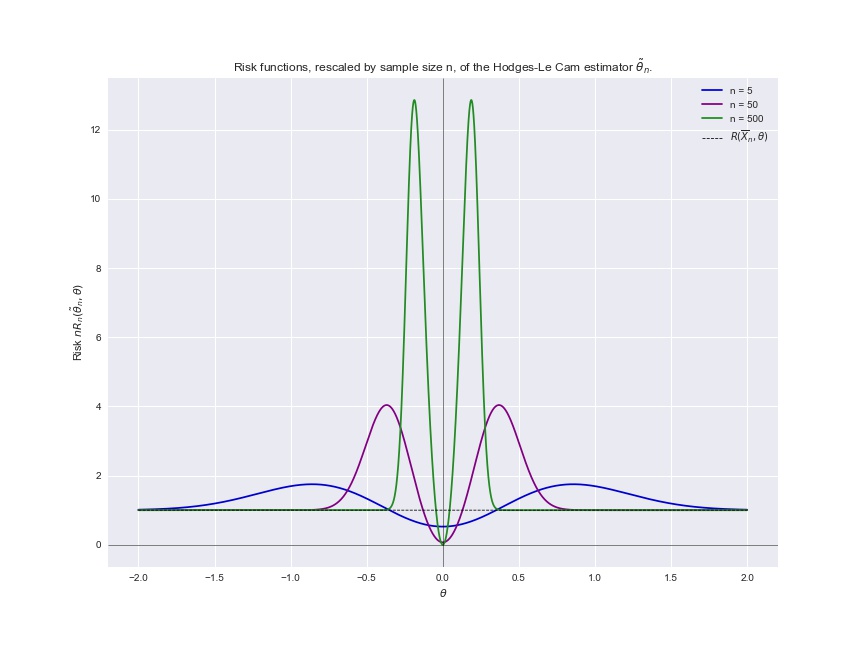
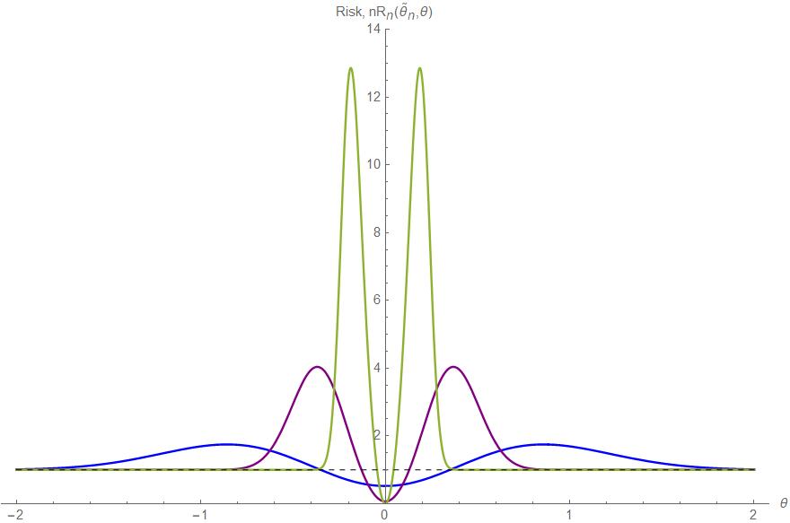
We will now derive the risk of the Hodges-Le Cam estimator under squared error loss and examine its behaviour.

In statistics, recall that one way of conceptualising the quality of an arbitrary estimator \(\hat{\theta}_n\) is through an informal notion of proximity. That is, we want to formalise the question, “how far away is the estimator \(\hat{\theta}_n\) from the true parameter \(\theta\)?”. We can do so formally using a loss function, \(L: \Theta \times \Theta \rightarrow \mathbb{R}^+\).

We now have to formally specify what we mean when we say “how far away”. In doing so, we will be encoding how we want to penalise deviations of the estimator \(\hat{\theta}_n\) from the true parameter \(\theta\). In this instance, we will use squared error loss,

The squared error loss function is ubiquitous in statistics and machine learning, and there are a few intutive points to note about its form. Firstly, the squaring of the deviation \((\hat{\theta}_n - \theta)\) means that we are indifferent to whether the estimator \(\hat{\theta}\) overestimates or underestimates the true parameter \(\theta\), we only care about the magnitude of the deviation. Secondly, that the deviations are squared means that we penalise the magnitude of the deviation in a quadratic, i.e. non-linear fashion.

Now where the notion of the risk of an estimator comes in, is in the fact that we are not only interested in the performance of an estimator \(\hat{\theta}_n\) on one data set, rather, we are interested in how this estimator performs over many hypothetical data sets. To capture this idea, we carry out averaging, and so the risk of an estimator is the expectation of the loss function, and under squared error loss, this is

With these elements introduced we can now proceed. Expanding the risk of the Hodges-Le Cam estimator, using linearity of expectation, we have that

which is a function of the mean and the second moment of the estimator \(\tilde{\theta}_n\). We now split the derivation up into two pieces:

1. Deriving the mean \(\mathbb{E}[\tilde{\theta}_n]\) of the estimator.

2. Deriving the second moment \(\mathbb{E}[\tilde{\theta}_n^2]\) of the estimator.

3. Combine the results to yield the risk \(nR_n(\tilde{\theta}_n, \theta)\).

Step 1. The mean \(\mathbb{E}[\tilde{\theta}_n]\) of the estimator.

The key to note here is that the estimator \(\tilde{\theta}_n\) is a mixed continuous and discrete random variable. Using the law of total probability, we have that

In order to evaluate this, we can use the fact that for a general random variable \(Y\) and for \(P(A) > 0\),

Setting \(Y = \bar{X}_n \sim N(\theta, 1/n)\), defining the set \(A = \{(\infty, -n^{-1/4}) \cup (n^{-1/4}, \infty) \}\), and noting the cancellation of \(P(A)\), we have that the mean of the estimator simplifies to

where \(f_Y(y)\) is the probability density of \(Y \sim N(\theta, 1 / n)\),

We now evaluate both definite integrals in general, and denoting them \(I_1(a, b)\), we have that

We now rewrite this integral in the following way:

For integral \((i)\), we can rewrite it with a view to making the substitution \(s(y) = -n(y - \theta)^2 /2\), and \(s'(y) = n(y - \theta)\) to simplify as follows,

Where the bounds of integration are \(s_2 = \max\{s(b), s(a)\}\) and \(s_1 = \min\{s(b), s(a)\}\).

For integral \((ii)\), we can rewrite and simplify it as follows,

Where we have used the fact that the integral on the right hand side of the first equality is just the area under the probability density \(f_Y(y)\) of \(Y \sim N(\theta, 1/n)\), and standardised to evaluate the integral in terms of the standard normal cumulative distribution function \(\Phi(t) = \int^{t}_{-\infty} \exp(-u^2) du\).

Now we have derived general expressions, we can evaluate them for the lower interval \(A_l = (\infty, -n^{-1/4})\) and upper interval \(A_u = (n^{-1/4}, \infty)\).

Beginning with the lower interval \(A_l\) where \(a = -\infty\) and \(b = -n^{-1/4}\), for integral \((i)\), we have that

Where we have used the fact that \(\lim_{y \rightarrow -\infty} s(y) = 0\). For integral \((ii)\), we have that

Where we have used the fact that \(\lim_{t \rightarrow -\infty} \Phi(t) = 0\).

For the upper interval \(A_u = (n^{-1/4}, \infty)\), we can conduct similar computations using the fact that \(\lim_{y \rightarrow \infty} s(y) = 0\); as well as properties of the standard Normal CDF \(\lim_{t \rightarrow \infty} \Phi(t) = 1\) and \(\Phi(-t) = 1 - \Phi(t)\).

Putting this all together, we have that for the lower interval \(A_l\) and the upper interval \(A_u\),

Hence the mean of the estimator is

Step 2. The second moment \(\mathbb{E}[\tilde{\theta}_n^2]\) of the estimator.

We have that

where \(f_Y(y)\) is the probability density of \(Y \sim N(\theta, 1/n)\), as before. We now evaluate both definite integrals in general, and denoting them both as \(I_2(a, b)\) we have that

Using a similar principle as before, we rewrite the integral in the following way:

For integral \((i)\), we carry out integration by parts, which is the result that \(\int uv' = uv - \int u'v\). Using the antiderivative derived in the previous section, and omitting the constant of integration, we identify

and also \(u(y) = y\) and \(u'(y) = 1\). We then have that the general form of integral \((i)\) is

where simplifications arise using the same arguments about \(f_Y(y)\) as in the previous section.

For integral \((ii)\) we can specify it in terms of the results from the previous section, that is,

At this stage, we defer evaluating integral \((ii)\) and only evaluate integral \((i)\) for the lower and upper intervals \(A_l = (-\infty, -n^{-1/4})\) and \(A_u = (n^{-1/4}, \infty)\).

For the lower interval \(A_l\), with \(a = -\infty\) and \(b = -n^{-1/4}\), evaluating the first term of integral \((i)\) yields

This is because

which is due to the fact that the term in the numerator, \(-y \rightarrow \infty\) at a linear rate, whereas the dominant term \(\exp(-n(y - \theta)^2/2) \rightarrow 0\) as \(y \rightarrow -\infty\) at an exponential rate.

For the second term in integral \((i)\), we have that

again because of the property of the standard normal cumulative distribution that \(\lim_{t \rightarrow - \infty} \Phi(t) = 0\).

For the upper interval \(A_u = (n^{-1/4}, \infty)\) and the first term in integral \((i)\) we can use the same argument that the rate at which \(-y \rightarrow - \infty\) is linear, whereas the dominant term \(\exp(-n(y - \theta)^2/2) \rightarrow 0\) at an exponential rate. For the second term in integral \((i)\), we similarly use properties of the standard normal cumulative distribution function that \(\lim_{t \rightarrow \infty} \Phi(t) = 1\) and \(\Phi(-t) = 1 - \Phi(t)\).

Defining both terms in the evaluation of integral \((i)\) for the lower interval \(A_l\) and \(A_u\) as \(c_l\) and \(c_u\), we have that

Hence the second moment of the estimator is

Step 3. Combine results to get the rescaled risk \(nR_n(\tilde{\theta}_n, \theta)\).

We now rescale the risk by the sample size \(n\) to get

Using the results we derived in previous sections, we have

Substituting the expressions we derived and simplifying, we have that

We can compress the notation by defining

Our final expression for the rescaled risk of the Hodges-Le Cam estimator is therefore

• Check the domain and range of estimators as functions formally.
• Assess whether to bundle the part about point estimation into an Appendix, or to include at beginning.
• Information on substitution trick.
• Check inequality/equality signs, and interval open/closed.

# Import modules.
import numpy as np
import matplotlib.pyplot as plt
from scipy.stats import norm
plt.style.use('seaborn')
plt.rcParams['figure.figsize'] = (12, 9)

# Risk under squared error loss of the Hodges-Le Cam estimator.
def risk_hodges_estimator(theta, sample_size):
    n = sample_size
    w1 = ((n ** 0.25) + theta * np.sqrt(n)) / np.sqrt(2)
    w2 = ((n ** 0.25) - theta * np.sqrt(n)) / np.sqrt(2)

    risk = ((n * (theta ** 2))
            + (w1 / np.sqrt(np.pi)) * np.exp(-(w1 ** 2))
            + ((1 - n * (theta ** 2)) * norm.cdf(-w1 * np.sqrt(2)))
            + (w2 / np.sqrt(np.pi)) * np.exp(-(w2 ** 2))
            + ((1 - n * (theta ** 2)) * norm.cdf(-w2 * np.sqrt(2))))

    return risk

# Plotting wrapper.
def generate_plots():
    theta_range = np.linspace(-2, 2, num=100000)
    sample_sizes = [5, 50, 500]

    fig, ax = plt.subplots(figsize=(12,10))

    # Plot the risk functions for n = 5, 50, 500.
    ax.plot(theta_range, risk_hodges_estimator(theta_range, 5),
            label='n = 5', color='mediumblue')

    ax.plot(theta_range, risk_hodges_estimator(theta_range, 50),
            label='n = 50', color='purple')

    ax.plot(theta_range, risk_hodges_estimator(theta_range, 500),
            label='n = 500', color='forestgreen')

    # Plot the constant risk of the sample mean as a reference.
    ax.plot(theta_range, np.ones((theta_range.shape[0],)),
            linestyle='dashed', lw=0.8, color='black',
            label=r'$R(\overline{X}_n, \theta)$')

    # Annotations.
    ax.axvline(0, 0, 1, color='k', lw=0.5)
    ax.axhline(0, 0, 1, color='k', lw=0.5)
    ax.set_title('Risk functions, rescaled by sample size n, of '
                 + 'the Hodges-Le Cam estimator' + r' $\tilde{\theta}_n$.')
    ax.set_xlabel(r'$\theta$')
    ax.set_ylabel('Risk ' + r'$nR_n(\tilde{\theta}_n , \theta)$')
    ax.legend()

# Generate plots.
generate_plots()